
PLC response time is the elapsed time between a defined field event and the required output or machine action. It includes more than the processor’s scan time: sensor behavior, input filtering, communication, task scheduling, output hardware and the actuator can all contribute. Define the start and end points first, allocate a timing budget to the complete chain, and verify it under realistic operating conditions. A fast average scan does not establish a guaranteed machine response. For cabinet acceptance, the useful question is whether the complete installed system consistently meets the process requirement, including its slowest permitted operating condition.
Define the event and the required result
A timing requirement needs two observable boundaries. “Respond quickly to a sensor” is incomplete. State whether timing starts when an object reaches a sensing position, when the sensor switches electrically or when a controller receives a message. State whether the endpoint is an output voltage change, contactor feedback, valve movement or the final process condition. Different boundaries produce different results, even when engineers are discussing the same machine.
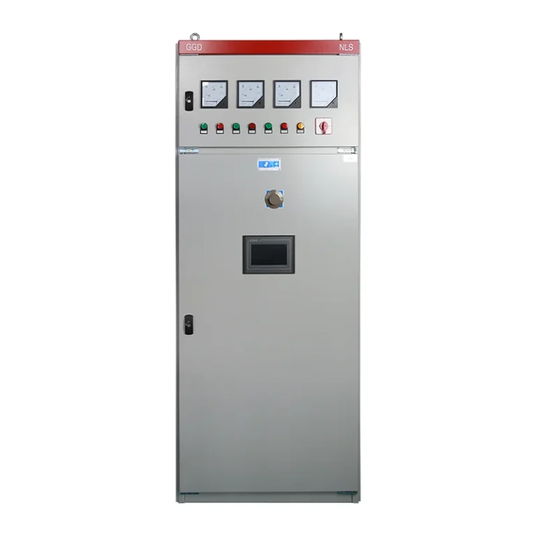
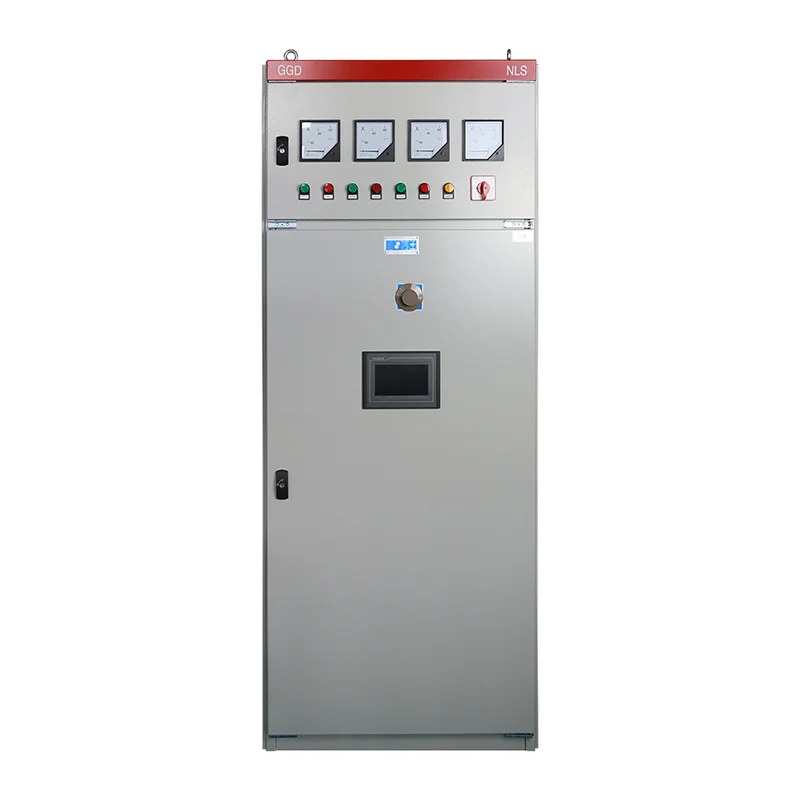
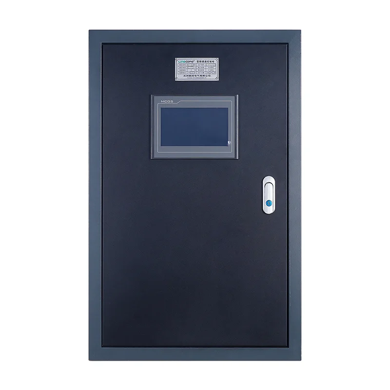
For a PLC control cabinet for industrial automation, include these boundaries in the functional specification and acceptance plan. A cabinet photograph establishes neither the processor model nor the installed input and output response characteristics. Obtain the actual hardware schedule, network topology and program revision. A timing promise should refer to those supplied components and the agreed test conditions. Use the PLC cabinet overview for the broader architecture; this article concentrates on proving timing performance.
Consider a conveyor diverter as a hypothetical planning case. An output may energize within the allocated electrical time while the pneumatic actuator arrives late because air pressure is low. Reporting only the controller’s output transition would miss the operational problem. Conversely, measuring from object arrival includes sensor geometry and detection distance, which cannot be attributed entirely to the PLC. Choose boundaries that answer the actual acceptance question and label every trace accordingly.
Understand where scan time fits
A conventional cyclic controller repeatedly obtains input information, evaluates its logic and updates outputs. The exact sequence, process-image behavior and communication arrangements depend on the controller and task configuration. The PLCtalk scan-cycle textbook chapter explains the basic cyclic model. Treat that model as an introduction, then use the supplied platform documentation to establish whether local inputs, remote inputs and interrupt tasks follow the same timing assumptions.
The arrival phase of an event matters. A signal that changes just after the relevant input update may wait longer than one that changes just before it. A program may also intentionally wait for a state transition, a timer or another permissive. Do not describe all of that waiting as execution time. Record the task period, observed execution time and relevant update intervals separately so that an unexpectedly slow result has a traceable explanation.
The RealPars guide to measuring PLC application performance discusses monitoring cycle statistics and testing the effect of optimization. Current, average and maximum observations answer different questions. A maximum seen during a short test is still only an observed maximum within that test. It is not automatically a guaranteed upper bound for every workload or future software revision.
Build a sensor-to-actuator timing budget
Allocate time to distinct stages before selecting hardware or changing software. The table below is an original project-planning framework based on the cyclic-control principles discussed above. Insert values only after checking the actual device documents and measurement method. Use the same units throughout and separate specified limits, configured intervals and measured results. A blank or unknown item should remain visible rather than being silently treated as zero.
| Stage | What to establish | Evidence for acceptance |
|---|---|---|
| Sensor and interface | Detection delay, switching behavior and signal duration | Device specification and field test |
| Input processing | Filter configuration and module response | Module identity, settings and trace |
| Data transfer | Local or remote update and communication loading | Actual topology and configured intervals |
| Controller task | Scheduling, execution and logic-dependent waiting | Program revision and diagnostic record |
| Output processing | Update behavior and output-device delay | Output type and observed transition |
| Final actuator | Travel, release or process completion time | Field measurement under defined conditions |
For an illustrative budget, suppose a non-safety process allocates 4 milliseconds to sensing and input processing, 18 milliseconds to data transfer and controller action, 6 milliseconds to the output chain and 42 milliseconds to actuator travel. The arithmetic total is 70 milliseconds. These are hypothetical allocations, not typical device ratings or a LINECOME performance claim. If the process permits 90 milliseconds, the remaining 20 milliseconds is only a planning margin until every stage and operating condition has been validated.
Write the calculation as T_total = T_sensor_input + T_transfer_control + T_output + T_actuator, with all terms in milliseconds. Avoid counting the same delay twice: a manufacturer’s end-to-end module figure may already include filtering, while a controller response specification may include particular I/O assumptions. Conversely, do not omit remote updates merely because the CPU is fast. Explain the boundaries of each term next to the calculation.
Check short events separately from overall delay
A response-time target does not guarantee that every short pulse will be detected. Signal duration, input filtering, module acquisition and task access all affect capture. An input may turn on and off between observations, leaving no event for ordinary cyclic logic to process. If a process depends on brief pulses, identify whether the application needs a supported pulse-capture feature, a high-speed input or another architecture. Verify that capability on the exact supplied hardware.
Do not solve pulse loss by automatically removing every filter. Filters can prevent unwanted transitions from contact chatter or interference. The right configuration must reject the unwanted signal while preserving the valid event and meeting the allowed response. Use the PLC input debounce guide for that separate signal-conditioning decision. Record the final filter setting in the timing test because changing it can alter both event capture and delay.
A simulated internal bit is useful for checking program flow, but it bypasses the physical input chain. Likewise, watching a tag on a programming laptop does not establish the timestamp of the field event: display refresh and communication add their own behavior. Keep software tests and physical response tests distinct. A complete handover can include both, provided each result states what was actually exercised.
Measure the chain with repeatable boundaries
Plan measurement connections, equipment and personnel before testing. Work on electrical systems requires suitable qualification, isolation and task-specific precautions. Where relevant, the OSHA electrical work-practice requirements provide a public reference; the site’s applicable rules and jurisdiction govern the actual work. Do not move probes or force outputs casually on a running machine merely to obtain a timing trace.
A useful test captures the initiating signal and the agreed endpoint on a common time base. Document instrument identification, sampling settings and how the endpoint is detected. If different logging systems supply the timestamps, establish clock synchronization and uncertainty before subtracting them. Controller logs, network captures and external measurements can complement each other, but their clock values should not be assumed directly comparable.
Repeat the event at varied phases relative to the controller task rather than accepting one favorable sample. Include the agreed production workload, communications, alarm activity and simultaneous device operations. Record the number of trials, the minimum and maximum observations and the acceptance threshold. Choose the test coverage according to process risk and engineering requirements; this article does not prescribe a universal sample count or confidence level.
Investigate the largest contributor first
When a response misses its target, compare the stage observations with the budget. A slow actuator may require mechanical or pneumatic investigation. A delayed remote input may require network and update review. A timer deliberately holding the sequence needs a functional review rather than a faster CPU. This approach avoids spending effort on processor execution when most of the delay occurs elsewhere.
Output technology also matters. An interposing relay or contactor has a physical operating and release process. Suppression components can affect release behavior. The PLC relay output suppression guide discusses that interface boundary. Do not remove suppression or substitute an output type without checking switching duty, device compatibility and the resulting acceptance requirements. The timing benefit of a change must be demonstrated together with reliable electrical operation.
If program changes are justified, preserve a tested backup and compare function before and after optimization. Moving logic into a faster task can introduce data-consistency or sequencing questions. Reducing a communication interval may increase traffic. Record the intended benefit, review the platform constraints and rerun the relevant functional and timing tests. A smaller diagnostic number is useful only if the machine still behaves correctly.
Separate ordinary control from safety response
A normal PLC response test is not evidence that a safety function meets its required performance. Safety applications need the appropriate components, architecture, validation and documented total response under the applicable standards. Mechanical stopping time and protective-distance calculations may be part of that separate assessment. Do not reuse the illustrative timing budget above as a safety calculation.
State this boundary in the inquiry and acceptance documents. If the customer asks for emergency-stop or protective-device response, identify the safety-function owner and the required validation scope. An ordinary machine-control sequence and a safety shutdown may share a cabinet while requiring different evidence. Keeping the scopes explicit prevents a general FAT timing result from being misused as a safety approval.
Put timing evidence in the cabinet handover
The final record should identify the initiating event, endpoint, operating mode, hardware and software revisions, settings, workload and instruments. Include the budget, the traces, the observed range, the acceptance decision and unresolved conditions. Record whether testing used real field devices or simulated signals. Retain the tested program and parameter set so future changes can be assessed against the accepted configuration.
For a quotation, send the required response, valid pulse duration, sensor and actuator types, local or remote I/O arrangement and expected network workload. Ask the cabinet supplier to identify what is included in the promised timing boundary. Agree how response will be demonstrated at FAT and which field-dependent items require site acceptance. This turns “fast PLC” into a measurable project requirement.
Further learning: the PLC control chain
The RealPars lesson below introduces how a PLC works. Use it to understand the role of inputs, logic and outputs before reviewing the timing budget. It does not specify the response of the cabinet pictured in this article or replace testing of the installed hardware and program.
Video by RealPars. Watch PLC Basics | Programmable Logic Controller on YouTube.
Frequently asked questions
Is PLC scan time the same as machine response time?
No. Scan time describes a controller execution cycle, while the machine response also depends on the defined sensor, communication, output and actuator boundaries.
Can average scan time prove a maximum response guarantee?
No. The guarantee needs an engineering basis and validation under the agreed conditions. Average scan time can conceal occasional delays and excludes other parts of the field chain.
Will a faster CPU always solve a missed timing target?
No. First identify the dominant delay. Input filtering, remote updates, deliberate sequencing and actuator movement may limit performance even when processor execution is short.