
A useful VFD energy savings calculation compares measured electricity use before and after speed control across the actual annual operating profile. For centrifugal fans and pumps in suitable friction-dominated systems, the affinity-law cube relationship provides an initial estimate of shaft-power reduction. It is not a guaranteed reduction in electrical input. Include motor and drive efficiency, static head or pressure requirements, minimum operating speed, annual hours and the existing throttling method before converting that estimate into annual kWh, cost savings and payback.
This guide focuses on calculations for HVAC fans and centrifugal water pumps. For terminology and application context, begin with our HVAC VFD guide. Constant-torque machinery, positive-displacement pumps and hoists require different load models; applying a fan’s cube relationship to those loads can seriously exaggerate the result.
Start with the existing system, not the motor nameplate
A 15 kW motor nameplate normally identifies rated mechanical output, not the electricity the installation continuously consumes. Actual electrical input depends on shaft load and efficiency. A partly loaded motor may draw substantially less power than its rated output suggests. Measure real input kW with suitable equipment and record the corresponding airflow, water flow, pressure and control position.
Document what currently regulates the process. A fixed-speed fan with dampers, a pump with a throttling valve, inlet guide vanes, bypass flow and simple on/off cycling produce different baselines. A calculation that assumes full electrical power whenever the system is enabled may overstate savings when the existing controls already reduce power or runtime.
The US Department of Energy’s Uniform Methods Project chapter on variable frequency drives provides an evaluation framework for estimating savings from these projects. Use a consistent boundary: include the same fan or pump service, the same relevant auxiliaries and comparable operating conditions on both sides of the comparison.
Use affinity laws as a screening tool
For the same centrifugal machine with unchanged impeller diameter, corresponding operating points are commonly approximated by Q₂/Q₁ = N₂/N₁, H₂/H₁ = (N₂/N₁)² and Pshaft,₂/Pshaft,₁ = (N₂/N₁)³. Q is flow, H is head or pressure, N is shaft speed and Pshaft is mechanical shaft power. The power relationship is most useful for systems where frictional resistance dominates and the operating points remain suitable.
At 80% speed, the ideal shaft-power ratio is 0.8³ = 0.512, corresponding to a 48.8% reduction from the reference shaft-power point. This says nothing yet about measured input kW, and it is not a universal 48.8% electricity-saving promise. The DOE’s Adjustable Speed Pumping Applications tip sheet explains the useful relationship and its limited-static-head context.
| Speed ratio | Ideal flow ratio | Ideal head ratio | Ideal shaft-power ratio |
|---|---|---|---|
| 100% | 100% | 100% | 100% |
| 90% | 90% | 81% | 72.9% |
| 80% | 80% | 64% | 51.2% |
| 70% | 70% | 49% | 34.3% |
Table values are calculated from the affinity relationships above for corresponding points. They are screening values, not predictions for a particular building. Shaft rpm is the preferred input. An output-frequency ratio can approximate speed ratio for an induction motor in a suitable operating range, but slip, control mode and load affect the correspondence.
Check whether static head or minimum pressure changes the model
In a pump lifting water between open tanks, the system must overcome elevation even at low flow. Reducing speed shifts the pump curve downward; below a certain speed, the pump may no longer develop enough head to produce useful flow. Assuming that flow always falls directly with speed can therefore be wrong.
Use the pump curve and system curve to find each proposed operating point. Check available suction conditions, minimum continuous flow, motor cooling and the equipment’s acceptable operating region. For a fan, verify the required duct pressure, terminal behavior and ventilation needs. A building cannot trade away required airflow simply because a lower speed gives an attractive spreadsheet result.
The DOE’s Improving Pumping System Performance sourcebook explains why the complete pumping system matters. For early project screening, label a cube-law estimate as preliminary. For a purchasing decision, replace it with validated operating points or measured test results whenever system characteristics make the approximation doubtful.
Convert shaft power to electrical input correctly
If the model begins with shaft power, estimated electrical input is Pin = Pshaft / (ηmotor × ηdrive), with efficiencies entered as decimals. For a line-fed baseline without a drive, use the relevant baseline efficiency and equipment boundary. Evaluate efficiency at the actual operating point; a motor’s full-load efficiency does not necessarily describe low-speed, lightly loaded service.
If the baseline already uses measured line-side input kW, do not divide that number by motor efficiency again. That would count a loss twice. Similarly, a manufacturer’s stated drive efficiency at one load point should not automatically be applied at every point in the operating profile. Ask for appropriate loss or efficiency data for the selected voltage, frame and duty.
Compare the resulting values at equal useful service. If the proposed controls also eliminate unnecessary hours, record that as a separate scheduling improvement. Combining a speed reduction, a runtime reduction and a changed production demand without identifying each contribution makes the final savings hard to verify.
A worked annual kWh and payback example
Assume a hypothetical fan operates for 4,000 hours per year. The existing system consumes a measured 12.0 kW in each of three representative demand bands. A validated retrofit assessment predicts 12.3 kW at full demand, 6.8 kW at medium demand and 3.8 kW at low demand. These are assumed electrical-input values for teaching the calculation, not measured LINECOME project results. They already include the proposed motor and drive losses.
| Demand band | Annual hours | Existing input | Proposed input | Annual reduction |
|---|---|---|---|---|
| High | 1,000 h | 12.0 kW | 12.3 kW | −300 kWh |
| Medium | 2,000 h | 12.0 kW | 6.8 kW | 10,400 kWh |
| Low | 1,000 h | 12.0 kW | 3.8 kW | 8,200 kWh |
| Total | 4,000 h | 48,000 kWh/year | 29,700 kWh/year | 18,300 kWh/year |
For each band, annual savings = (existing kW − proposed kW) × annual hours. Add the bands to obtain 18,300 kWh/year, or 38.125% of the example baseline. The high-demand band shows a small penalty because the example includes added drive losses when no useful speed reduction is available. Retaining that penalty makes the estimate more credible than omitting inconvenient operating periods.
At an illustrative flat energy price of US$0.12/kWh, annual energy-cost savings are 18,300 × 0.12 = US$2,196. If total installed project cost is US$7,500, simple payback is 7,500 / 2,196 = 3.42 years. Actual tariffs may include demand charges and time-of-use rates. Calculate those separately from the energy charge; reduced kWh does not guarantee the same percentage reduction in total bills.
Include the costs that make a retrofit usable
Installed cost should include the drive, enclosure or cabinet, protection, appropriate filtering where required, controls, sensors, wiring, engineering, installation, shutdown work and commissioning. A purchase price alone does not represent the investment needed to achieve dependable service. Include recurring costs if they materially affect the decision, while keeping speculative maintenance savings separate from the core energy estimate.
Review motor insulation suitability, cable length, grounding, operating-speed range, cooling and the application’s current requirement before selecting hardware. Use our AC drive cabinet-planning guide for the installation discussion. Energy savings depend on the load and control strategy; installing a drive without allowing useful speed reduction may add losses without delivering the expected benefit.
Build a load profile that reflects the full year
Log representative weekdays, weekends, production shifts and seasonal conditions. A short winter test may miss summer cooling demand, while one busy shift can exaggerate annual full-load hours. Match the annual hours in all demand bands to realistic schedules. Standby periods and stopped hours should be explicit rather than quietly counted as operating time.
Test at several safe speeds and record input kW alongside flow and pressure. Use compatible instruments and qualified personnel; ordinary current readings alone do not establish real power in a drive system. Record sensor calibration and control setpoints so future comparisons can distinguish a genuine efficiency improvement from a changed service requirement.
Check sensitivity before approving the project. Recalculate with fewer reduced-speed hours, a higher installed cost and a lower electricity price. If the project only pays back under the most optimistic assumptions, gather more evidence. A transparent range is more useful than an apparently precise figure built on weak inputs.
Specify the drive around the operating requirement
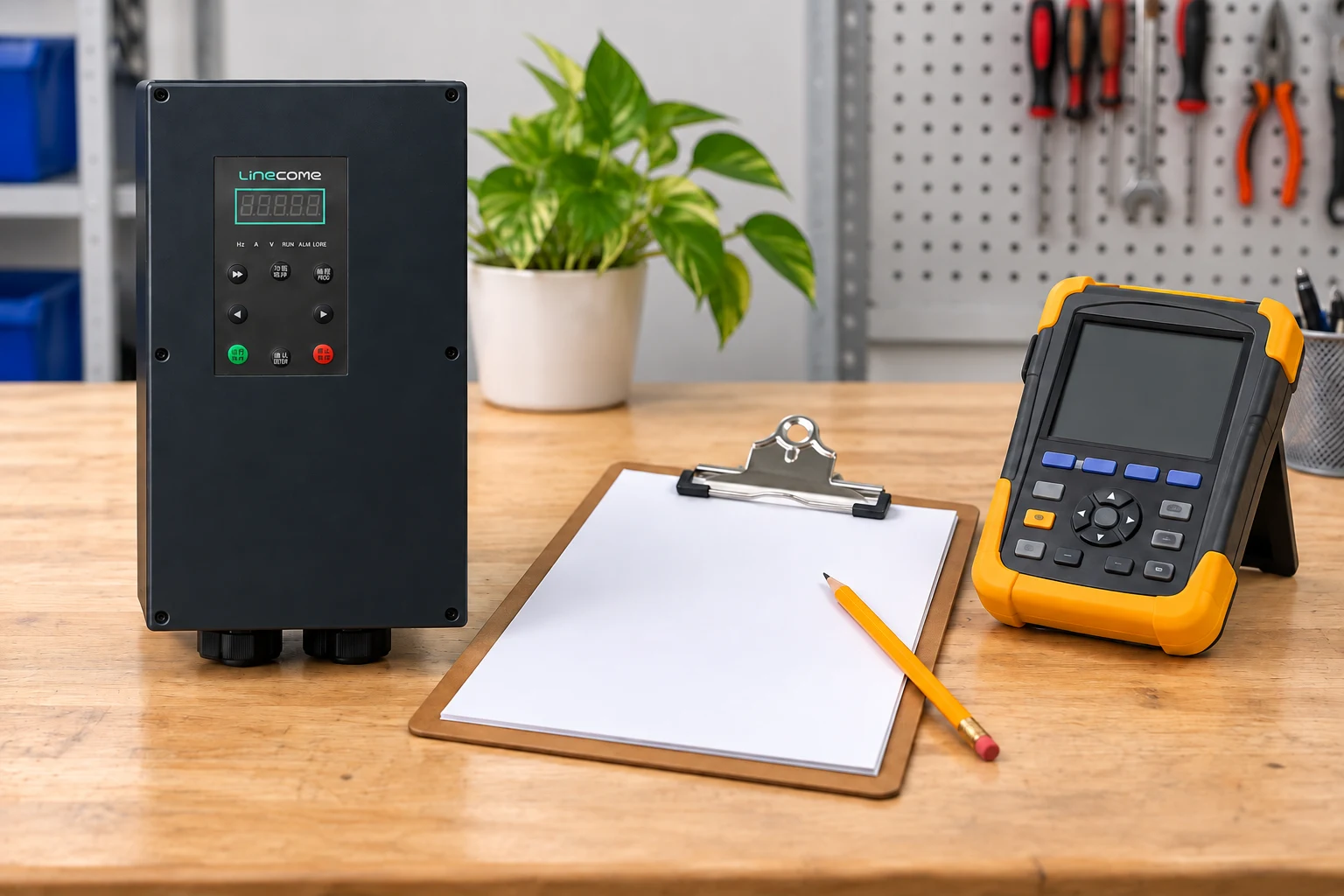
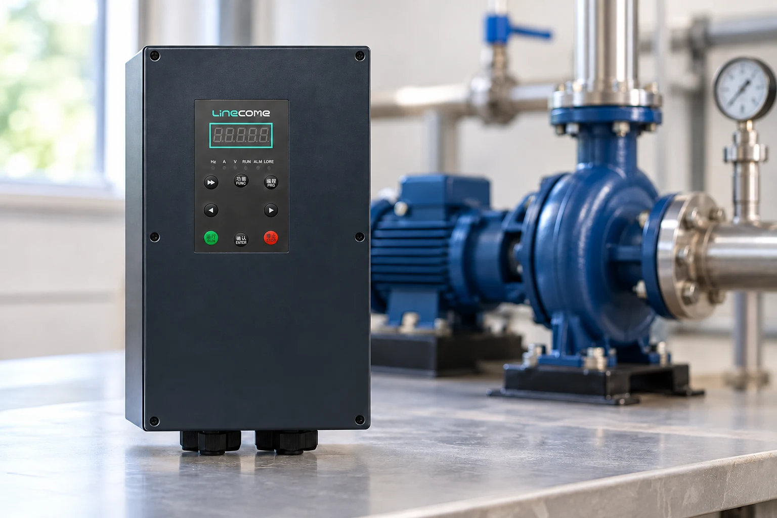
The LINECOME LNC820D range is one starting point for discussing a fan or pump application requiring an enclosed drive. Confirm the exact model’s environmental suitability, current rating and control functions with the supplier. Its product-family name does not establish suitability for every outdoor, wet or corrosive location, nor does it guarantee a particular saving.
Send the motor nameplate, supply details, load profile, existing controls, pump or fan curve, required flow and pressure, site environment and proposed communications interface. Ask for a duty-specific selection and commissioning scope. The LINECOME product hub helps compare the available families, while our overview of VFD benefits places energy reduction alongside control and mechanical considerations.
Verify savings after commissioning
Repeat input-power logging after the controls have stabilized. Compare like-for-like production or weather conditions, or apply a documented adjustment where conditions differ. Confirm minimum flow, pressure stability, comfort, process performance and safe operating limits before accepting the energy figure. Record final setpoints and retain the original baseline so future changes do not erase the evidence behind the investment.
The Engineering Mindset’s educational video below explains how frequency control changes motor operation. It provides background for the speed-control principle; the annual savings still need the site-specific measurements and calculations described in this article.
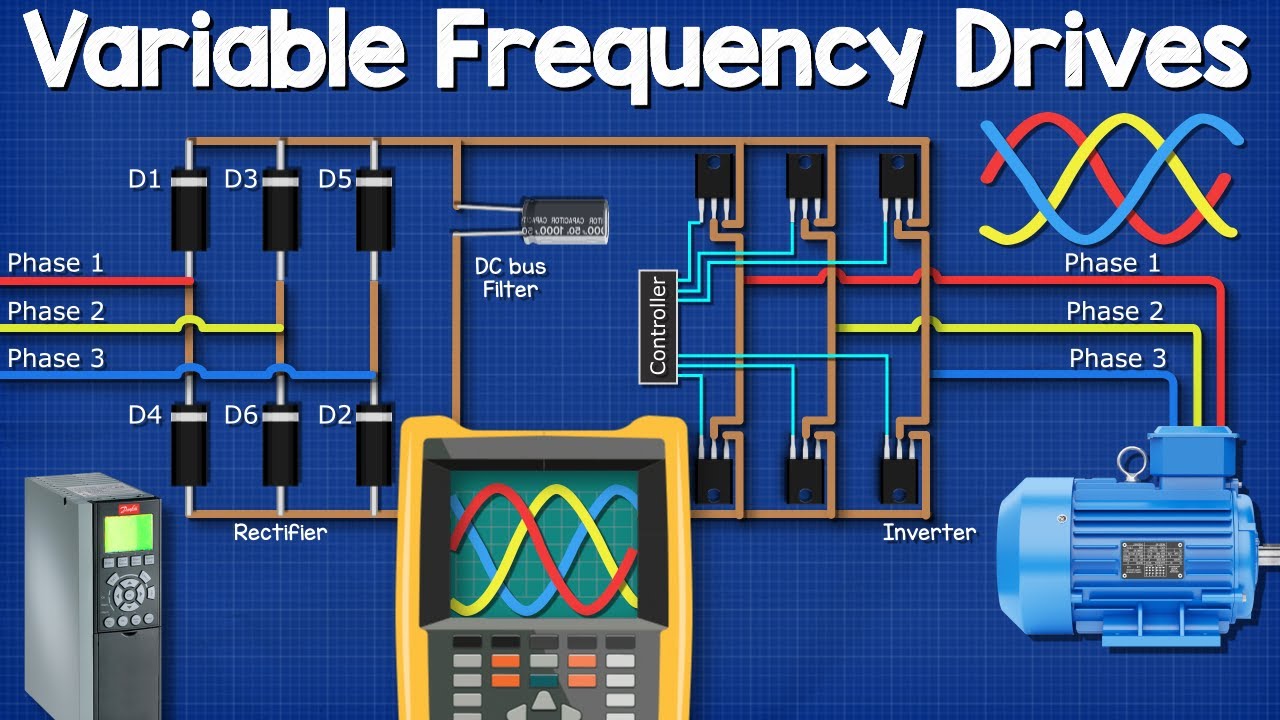
Watch the VFD explanation on YouTube.
Frequently asked questions
Does running at 80% speed always save 48.8% electricity?
No. That is an ideal shaft-power reduction for an applicable centrifugal-load model. Actual electricity savings depend on the system curve, existing control method, motor and drive losses, and operating hours.
Can motor rated kW replace a power measurement?
Not reliably. Rated motor kW normally describes mechanical output capacity. Use measured electrical input or a validated load-and-efficiency model for the baseline.
Can I use the cube law for a conveyor or hoist?
No. Those applications generally require a different torque and duty model. The fan and centrifugal-pump screening relationship should not be transferred to them.
What is the basic annual savings formula?
Add (baseline input kW minus proposed input kW) multiplied by annual hours for every representative operating band. Apply the appropriate energy tariff afterward and assess demand charges separately.